はじめに
iimonでエンジニアをしています。腰丸です。 SQLを触る際に、お世話になるINDEXですが、理解しているようで、実はよくわからないという方も多いのではないでしょうか。(自分は自信ないです) 今回は、SQLのINDEXについて、実際のデータを使ってB-treeの構造を確認しながら、理解を深めていきたいと思います。 弊社のサービスでは、MySQLを使用していますが、データの確認がしやすいため、今回はPostgreSQLを使用しています。
SQLのINDEX検索概要
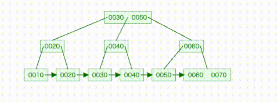
基本的なRDBでは、INDEXを貼ることで、効率のよい検索を実現しています。 SQLデータベースにおけるBツリーの検索構造は、 「ルートノード → ブランチノード → リーフノード」の階層構造でデータが管理されることが多いです。
- ルートノード: ツリーの最上位で検索の起点
- ブランチノード: データの分岐ポイント
- リーフノード: 実際のデータへのポインタ(インデックスエントリを持つ)
この構造により、条件に合致するデータの探索が効率的に行えます。
- イメージ図
実際のデータで見てみる
Dockerコンテナ
- docker-compose.yml
version: '3.8'

services:
  postgres:
    image: postgres:17
    container_name: postgres_pageinspect
    ports:
      - "5432:5432"
    environment:
      POSTGRES_USER: postgres
      POSTGRES_PASSWORD: postgres
      POSTGRES_DB: testdb
    volumes:
      - pgdata:/var/lib/postgresql/data

volumes:
  pgdata:
- 接続コマンド
docker exec -it postgres_pageinspect psql -U postgres -d testdb
データ準備
- テーブル定義
CREATE TABLE sample_table (
    id INT PRIMARY KEY,
    column1int int,
    column2varchar VARCHAR(255),
    created_at TIMESTAMP DEFAULT CURRENT_TIMESTAMP
);

CREATE INDEX idx_sample_column1int ON sample_table (column1int);
- データ投入(データの内容をみやすくするため、1000件程度に留めています)
import psycopg2

# PostgreSQLに接続する情報
db_config = {
    'host': 'localhost',
    'port': '5432',
    'dbname': 'testdb',
    'user': 'postgres',
    'password': 'postgres',
}

# SQL
insert_sql = "INSERT INTO sample_table (id, column1int, column2varchar) VALUES (%s, %s, %s);"
check_level_sql = "SELECT level FROM bt_metap('idx_sample_column1int');"

try:
    conn = psycopg2.connect(**db_config)
    conn.autocommit = True
    cur = conn.cursor()

    for i in range(1, 1000):
        # 1件ずつINSERT
        cur.execute(insert_sql, (i, i, f'Name_{i}'))

        cur.execute(check_level_sql)
        level = cur.fetchone()[0]
        print(f"Inserted {i} rows - Current B-Tree Level: {level}")

        if level >= 2:
            print(f"✅ B-Tree Level 2 に到達!行数: {i}")
            break

    cur.close()
    conn.close()

except Exception as e:
    print("❌ エラーが発生しました:", e)
データを見てみる
indexのメタデータを確認
# SELECT * FROM bt_metap('idx_sample_column1int');
 magic  | version | root | level | fastroot | fastlevel | last_cleanup_num_delpages | last_cleanup_num_tuples | allequalimage
--------+---------+------+-------+----------+-----------+---------------------------+-------------------------+---------------
 340322 |       4 |    3 |     1 |        3 |         1 |                         0 |                      -1 | t
(1 row)
説明
ルートページ番号 (
root)
インデックスの「入り口」であるページ番号が記載されています。検索はここから始まり、各リーフノードへの道しるべを持っています。
この内容によると、ルートページ番号は3です。高さ (
level)
B-Treeの層の深さ。1の場合、ルートノードの下に直接リーフノードがある「シンプルな2階層構造」になります。
B-Treeのルートノードを見てみる
- 3ページ目がルートノードで、1階層のB-Tree構造を持つことがわかったので、このルートノードの中身を見てみましょう。
SELECT * FROM bt_page_items('idx_sample_column1int', 3);


 itemoffset | ctid  | itemlen | nulls | vars |          data           | dead | htid | tids
------------+-------+---------+-------+------+-------------------------+------+------+------
          1 | (1,0) |       8 | f     | f    |                         |      |      |
          2 | (2,1) |      16 | f     | f    | 6f 01 00 00 00 00 00 00 |      |      |
          3 | (4,1) |      16 | f     | f    | dd 02 00 00 00 00 00 00 |      |      |

(3 rows)

 ```
補足
- 内部ノード(ルートノード/ブランチノード)のctidは“左端のダウンリンク”で、実際のデータ行を示しているわけではありません。
data列.
- リトルエンディアンという形式で、境界値となる値が格納されていました。(aarch64の場合)
- 10進数値はそれぞれ下記の内容になります。
- 6f 01 00 00 00 00 00 00 -> 0x016f = (0x01 * 256) + (0x6f) = (1 * 256) + (111) = 367
- dd 02 00 00 00 00 00 00 -> 0x02dd = (0x02 * 256) + (0xdd) = (2 * 256) + (221) = 733
- 10進数値はそれぞれ下記の内容になります。
ctid.
- 通常は、ctid は単に「インデックスエントリが指す先」のテーブルの行位置(= テーブルのブロック番号, スロット番号)を示しています。
- 内部ノードでは、インデックスの「左端のダウンリンク」を示しています。
リーフノードの内容を見てみる
- 右端以外のリーフノードの1行目は、「High Key」というもので、そのページ値がdataの値未満であることを示しています。(ctidも実際のデータ行を指していません)
リーフノード1
SELECT ctid, data, s.id, s.column1int, s.column2varchar FROM bt_page_items('idx_sample_column1int', 1) as b
LEFT JOIN sample_table s ON s.ctid = b.ctid;

  ctid   |          data           | id  | column1int | column2varchar
---------+-------------------------+-----+------------+----------------
 (2,1)   | 6f 01 00 00 00 00 00 00 |     |            |
 (0,1)   | 01 00 00 00 00 00 00 00 |   1 |          1 | Name_1
 (0,2)   | 02 00 00 00 00 00 00 00 |   2 |          2 | Name_2
 (0,3)   | 03 00 00 00 00 00 00 00 |   3 |          3 | Name_3
...
 (2,78)  | 6b 01 00 00 00 00 00 00 | 363 |        363 | Name_363
 (2,79)  | 6c 01 00 00 00 00 00 00 | 364 |        364 | Name_364
 (2,80)  | 6d 01 00 00 00 00 00 00 | 365 |        365 | Name_365
 (2,81)  | 6e 01 00 00 00 00 00 00 | 366 |        366 | Name_366
(367 rows)
リーフノード2
SELECT ctid, data, s.id, s.column1int, s.column2varchar FROM bt_page_items('idx_sample_column1int', 2) as b
INNER JOIN sample_table s ON s.ctid = b.ctid;

  ctid   |          data           | id  | column1int | column2varchar
---------+-------------------------+-----+------------+----------------
 (5,1)   | dd 02 00 00 00 00 00 00 |     |            |
 (2,82)  | 6f 01 00 00 00 00 00 00 | 367 |        367 | Name_367
 (2,83)  | 70 01 00 00 00 00 00 00 | 368 |        368 | Name_368
...
 (5,37)  | da 02 00 00 00 00 00 00 | 730 |        730 | Name_730
 (5,38)  | db 02 00 00 00 00 00 00 | 731 |        731 | Name_731
 (5,39)  | dc 02 00 00 00 00 00 00 | 732 |        732 | Name_732
(367 rows)
リーフノード3
SELECT ctid, data, s.id, s.column1int, s.column2varchar FROM bt_page_items('idx_sample_column1int', 4) as b
INNER JOIN sample_table s ON s.ctid = b.ctid;

  ctid   |          data           | id  | column1int | column2varchar
---------+-------------------------+-----+------------+----------------
 (5,40)  | dd 02 00 00 00 00 00 00 | 733 |        733 | Name_733
 (5,41)  | de 02 00 00 00 00 00 00 | 734 |        734 | Name_734
 (5,42)  | df 02 00 00 00 00 00 00 | 735 |        735 | Name_735
...
 (7,32)  | e5 03 00 00 00 00 00 00 | 997 |        997 | Name_997
 (7,33)  | e6 03 00 00 00 00 00 00 | 998 |        998 | Name_998
 (7,34)  | e7 03 00 00 00 00 00 00 | 999 |        999 | Name_999
(267 rows)
ノード別まとめ
This is a B-tree leaf page. All tuples that point to the table happen to be posting list tuples (all of which store a total of 100 6 byte TIDs). There is also a “high key” tuple at itemoffset number 1. ctid is used to store encoded information about each tuple in this example, though leaf page tuples often store a heap TID directly in the ctid field instead. tids is the list of TIDs stored as a posting list.
In an internal page (not shown), the block number part of ctid is a “downlink”, which is a block number of another page in the index itself. The offset part (the second number) of ctid stores encoded information about the tuple, such as the number of columns present (suffix truncation may have removed unneeded suffix columns). Truncated columns are treated as having the value “minus infinity”.
htid shows a heap TID for the tuple, regardless of the underlying tuple representation. This value may match ctid, or may be decoded from the alternative representations used by posting list tuples and tuples from internal pages. Tuples in internal pages usually have the implementation level heap TID column truncated away, which is represented as a NULL htid value.
Note that the first item on any non-rightmost page (any page with a non-zero value in the btpo_next field) is the page's “high key”, meaning its data serves as an upper bound on all items appearing on the page, while its ctid field does not point to another block. Also, on internal pages, the first real data item (the first item that is not a high key) reliably has every column truncated away, leaving no actual value in its data field. Such an item does have a valid downlink in its ctid field, however.
↑ pageinspectのctid、dataの扱いに関する補足
まとめ
| ノード種類 | itemoffset | data 列の意味 | ctid の意味 |
|---|---|---|---|
| ルート/中間 | 1 | “minus-infinity” ダウンリンク | 子ページへのダウンリンク(ブロック番号) |
| >1 | 子ページに含まれるキーの下限 (lower bound) | 子ページへのダウンリンク(ブロック番号) | |
| リーフ (非右端) | 1 | このページに含まれる全アイテムの上限キー (High Key) | 無効(ダミー) |
| リーフ (全ページ) | >1 | 実データ行の値 (column1int の値) | ヒープ上の行位置(テーブルの (block, slot)) |
B-Tree構造の図
                             [367, 733]
                             (Root Node)
                                |
  ┌─────────────────────────────────────────────────────────────┐
  │                                                             │
[1-366]                      [367-732]                       [733-999]
(Leaf Node 1)                (Leaf Node 2)                   (Leaf Node 3)
実行結果を見てみる
- まずは、単純なクエリで見てみます。
indexあり
EXPLAIN (ANALYZE, BUFFERS)
SELECT * FROM sample_table WHERE column1int = 100;

Index Scan using idx_sample_column1int on sample_table  (cost=0.28..8.29 rows=1 width=24) (actual time=0.102..0.103 rows=1 loops=1)
  Index Cond: (column1int = 100)
  Buffers: shared hit=3
- 検索フローイメージ
                ┌─────────┐
                │ Root    │   ← bt_page_items で見た “ルートノード”(ページ3)
                │ (page 3)│
                └────┬────┘
                     │ key = 100 を探索
                     ▼
              ┌──────────────┐
              │ Leaf Node    │
              │ (page 1)     │
              └──────┬───────┘
                     │ index entry → ctid=(0,100) →
                     ▼               ヒープの block 0 を指す
              ┌──────────────┐
              │ Heap Page    │   ← テーブルの実データを格納するページ
              │ (block 0)    │
              └──────────────┘
indexなし
EXPLAIN (ANALYZE, BUFFERS)
SELECT * FROM sample_table_no_index WHERE column1int = 100;

Seq Scan on sample_table_no_index  (cost=0.00..20.49 rows=1 width=24) (actual time=0.078..0.194 rows=1 loops=1)
  Filter: (column1int = 100)
  Rows Removed by Filter: 998
  Buffers: shared hit=8
- イメージ
┌───────────┐   ┌───────────┐   ┌───────────┐   ┌───────────┐
│ Heap page │   │ Heap page │   │ Heap page │   │ Heap page │
│ (block0)  │─▶│ (block1)  │─▶ │ (block2)  │─▶ │ (block3)  │
└───────────┘   └───────────┘   └───────────┘   └───────────┘
     │              │              │              │
     ▼              ▼              ▼              ▼
   Filter:       Filter:        Filter:        Filter:
 column1int=100? ...            ...            ...
     │              │              │              │
   match!        no match      no match      no match

┌───────────┐   ┌───────────┐   ┌───────────┐   ┌───────────┐
│ Heap page │   │ Heap page │   │ Heap page │   │ Heap page │
│ (block4)  │─▶│ (block5)  │─▶ │ (block6)  │─▶ │ (block7)  │
└───────────┘   └───────────┘   └───────────┘   └───────────┘
     │              │              │              │
     ▼              ▼              ▼              ▼
   Filter:      Filter:        Filter:      Filter:
 column1int=100? ...            ...          ...
     │              │              │              │
  no match       no match      no match      no match
- INDEXの有無で、検索の効率が大きく変わることがわかります。
Heap page(テーブルブロック)の最後に条件に合致するデータを足してみる
- ブロック7(既存のデータとは別のブロック)に条件に合致するデータが追加されることがわかります。
INSERT INTO sample_table (id, column1int, column2varchar) VALUES
(1000, 100, 'Alpha'),
(1001, 100, 'Beta');

SELECT ctid, * FROM sample_table WHERE column1int = 100;
  ctid   |  id  | column1int | column2varchar |         created_at
---------+------+------------+----------------+----------------------------
 (0,100) |  100 |        100 | Name_100       | 2025-05-26 13:23:54.382557
 (7,35)  | 1000 |        100 | Alpha          | 2025-05-26 16:11:46.098942
 (7,36)  | 1001 |        100 | Beta           | 2025-05-26 16:31:45.572123
(3 rows)
- EXPLAIN
EXPLAIN (ANALYZE, BUFFERS)
SELECT * FROM sample_table WHERE column1int = 100;

Index Scan using idx_sample_column1int on sample_table  (cost=0.28..8.29 rows=1 width=24) (actual time=0.044..0.050 rows=3 loops=1)
  Index Cond: (column1int = 100)
  Buffers: shared hit=4
- Buffers: shared hit=4となり、別ブロックのデータ読み取りが発生していることがわかります。
- 今回は、小件数のデータですが、大量のデータが存在する場合には、実データの分布もパフォーマンスに影響することが推測できます。
indexを貼っていない条件を足してみる
AND column2varchar = 'Alpha'の条件を追加して検索してみます。
EXPLAIN (ANALYZE, BUFFERS)
SELECT * FROM sample_table WHERE column1int = 100 AND column2varchar = 'Alpha';

Index Scan using idx_sample_column1int on sample_table  (cost=0.28..8.29 rows=1 width=24) (actual time=0.117..0.118 rows=1 loops=1)
  Index Cond: (column1int = 100)
  Filter: ((column2varchar)::text = 'Alpha'::text)
  Rows Removed by Filter: 2
  Buffers: shared hit=4
- Filter: ((column2varchar)::text = ‘Alpha’::text)が追加されていることから、
インデックス条件だけでは足りず、さらに実データ(Heap)を見て、 column2varchar = 'Alpha' のフィルターが走っていることがわかります。
複合INDEXを貼ってみる
- 複合INDEXを貼ることで、column1intとcolumn2varcharの両方の条件をインデックスでカバーできるようにします。
CREATE INDEX idx_sample_column1int_and_column2varchar ON sample_table (column1int, column2varchar varchar_pattern_ops);
- varchar_pattern_opsを指定することで、LIKE検索などのパターンマッチングに最適化されます。(本記事では触れません)
ルートノードを確認
SELECT * FROM bt_page_items('idx_sample_column1int_and_column2varchar', 3);

 itemoffset | ctid  | itemlen | nulls | vars |          data           | dead | htid | tids
------------+-------+---------+-------+------+-------------------------+------+------+------
          1 | (1,0) |       8 | f     | f    |                         |      |      |
          2 | (2,1) |      16 | f     | f    | 04 01 00 00 00 00 00 00 |      |      |
          3 | (4,1) |      16 | f     | f    | 09 02 00 00 00 00 00 00 |      |      |
          4 | (5,1) |      16 | f     | f    | 0e 03 00 00 00 00 00 00 |      |      |
(4 rows)
- data列の変換
| itemoffset | data | 16進表記 | 10進値 |
|---|---|---|---|
| 2 | 04 01 00 00 00 00 00 00 |
0x0104 |
260 |
| 3 | 09 02 00 00 00 00 00 00 |
0x0209 |
521 |
| 4 | 0e 03 00 00 00 00 00 00 |
0x030e |
782 |
- このルートノードは、column1intの値が260, 521, 782の境界値を持つことを示しています。
- あくまでcolumn1intの値が最初の検索の入口となることが推測できます。
リーフノードを確認
SELECT ctid, data, s.column1int, s.column2varchar FROM bt_page_items('idx_sample_column1int_and_column2varchar', 1) as b
JOIN sample_table s ON s.ctid = b.ctid;

  ctid   |                      data                       | column1int | column2varchar
---------+-------------------------------------------------+------------+----------------
 (1,1)   | 04 01 00 00 00 00 00 00                         |        150 | Name_150
 (0,1)   | 01 00 00 00 0f 4e 61 6d 65 5f 31 00 00 00 00 00 |          1 | Name_1
 (0,2)   | 02 00 00 00 0f 4e 61 6d 65 5f 32 00 00 00 00 00 |          2 | Name_2
...
 (0,97)  | 61 00 00 00 11 4e 61 6d 65 5f 39 37 00 00 00 00 |         97 | Name_97
 (0,98)  | 62 00 00 00 11 4e 61 6d 65 5f 39 38 00 00 00 00 |         98 | Name_98
 (0,99)  | 63 00 00 00 11 4e 61 6d 65 5f 39 39 00 00 00 00 |         99 | Name_99
 (7,35)  | 64 00 00 00 0d 41 6c 70 68 61 00 00 00 00 00 00 |        100 | Alpha
 (7,36)  | 64 00 00 00 0b 42 65 74 61 00 00 00 00 00 00 00 |        100 | Beta
 (0,100) | 64 00 00 00 13 4e 61 6d 65 5f 31 30 30 00 00 00 |        100 | Name_100
 (0,101) | 65 00 00 00 13 4e 61 6d 65 5f 31 30 31 00 00 00 |        101 | Name_101
...
 (1,108) | 01 01 00 00 13 4e 61 6d 65 5f 32 35 37 00 00 00 |        257 | Name_257
 (1,109) | 02 01 00 00 13 4e 61 6d 65 5f 32 35 38 00 00 00 |        258 | Name_258
 (1,110) | 03 01 00 00 13 4e 61 6d 65 5f 32 35 39 00 00 00 |        259 | Name_259
(262 rows)
- column1intの値が同じ場合に、column2varcharの値が昇順に並んでいることがわかります。
- column1intが同じ値であれば、column2varcharは近くに並んでいるため、効率的に検索可能であるということが推測できます。
複合INDEXを使ったクエリ実行
EXPLAIN (ANALYZE, BUFFERS)
SELECT * FROM sample_table WHERE column1int = 100 AND column2varchar = 'Alpha';

Index Scan using idx_sample_column1int_and_column2varchar on sample_table  (cost=0.28..8.29 rows=1 width=24) (actual time=0.587..0.590 rows=1 loops=1)
  Index Cond: ((column1int = 100) AND ((column2varchar)::text = 'Alpha'::text))
  Buffers: shared hit=3
- Index Cond: *1が表示され、Filterがなくなっていることがわかります。
- 複合INDEXを使用することで、column1intとcolumn2varcharの両方の条件をインデックスでカバーできるようになり、実データ(Heap)をフィルターする必要がなくなりました。
おわりに
すべてに目を通してはいないのですが、「開発者のためのSQLパフォーマンスの全て(https://use-the-index-luke.com/ja/sql/table-of-contents)」 というサイトが非常にわかりやすく、より発展的な内容を理解する参考になりました。 普段は意識することが少ないかもしれませんが、初歩的なINDEXの仕組みや効果をイメージする一助となれば幸いです。
ここまでお読みいただき、ありがとうございます。
弊社ではエンジニアを募集しております。
この記事を読んで少しでも興味を持ってくださった方は、ぜひカジュアル面談でお話ししましょう!
下記リンクよりご応募お待ちしております!
iimon採用サイト / Wantedly / Green
*1:column1int = 100) AND ((column2varchar)::text = 'Alpha'::text